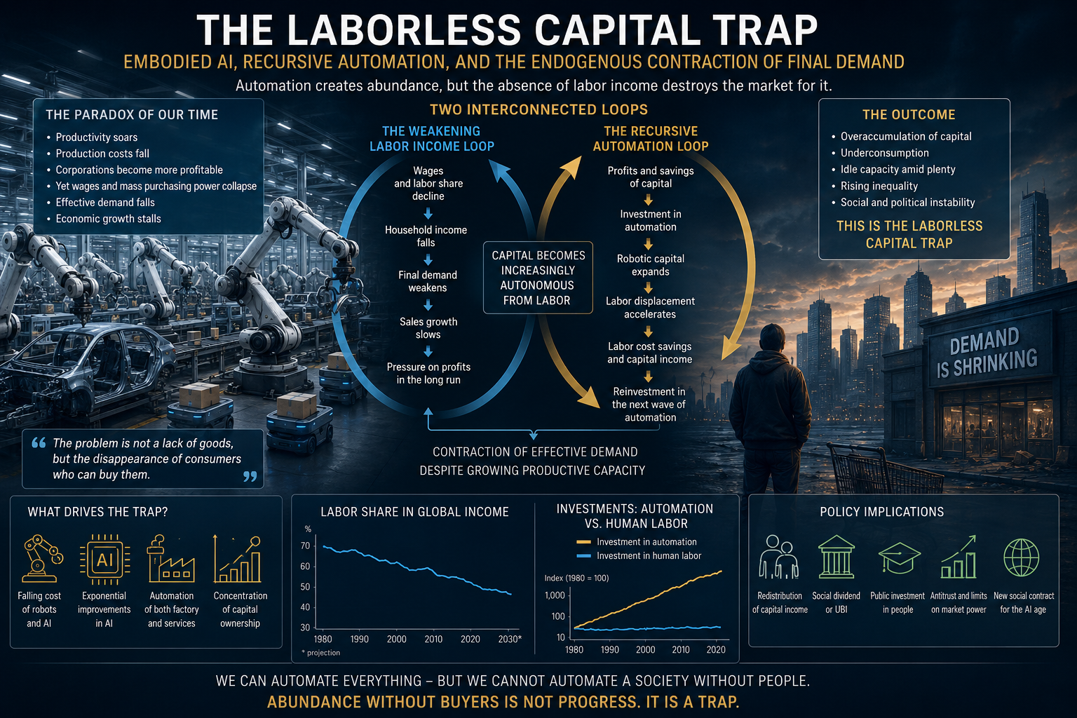
The Laborless Capital Trap: Embodied AI, Recursive Automation, and the Endogenous Contraction of Final Demand

17.08.2026

374
Embodied Artificial Intelligence, Recursive Automation, and the Endogenous Contraction of Final Demand
The Laborless Capital Trap: Embodied Artificial Intelligence, Recursive Automation, and the Endogenous Contraction of Final Demand
Authors
Abstract
This paper extends Falk and Tsoukalas’s (2026) model in The AI Layoff Trap, in which competitive firms automate more tasks than would maximize their joint profits because each firm captures the full labor-cost saving while bearing only part of the demand contraction generated by layoffs. In the original model, the investment channel is treated primarily as a possible mechanism for returning displaced income to the economy. This paper endogenizes the destination of that return and studies the case in which automation profits are reinvested predominantly in labor-substituting capital: software AI, industrial robots, autonomous logistics, robotic production lines, and other forms of embodied artificial intelligence.
A dynamic two-sector model is proposed that distinguishes the production of final goods from the production of automated capital itself. The model introduces the labor share in final-sector output, the labor content of investment, ownership concentration, the propensities of workers and capital owners to consume, and an endogenous decline in the cost of subsequent rounds of automation. Investment constitutes aggregate demand in national accounts, but need not restore household final demand: as the capital-goods sector is automated, its capacity to generate wage income converges toward zero. A recursive structure emerges in which labor-cost savings and capital income are reinvested in robotic capital, robotic capital displaces further labor, and the next round of automation becomes easier to finance and implement.
The following results are obtained. First, the marginal contribution of investment to final demand falls monotonically with the labor content of robot production and with the consumption propensity of increasingly concentrated capital owners. Second, productive capacity can persistently outgrow effective final demand, producing lower utilization, capital write-downs, and consolidation rather than an indefinitely expanding stock of unsold goods. Third, a sectoral monopolist does not eliminate the externality because it internalizes only the portion of expenditure contraction that falls on the sectors it owns. Fourth, ownership concentration simultaneously raises the share of profits available for automation and lowers the current consumption rate. In the post-labor limit, the problem becomes institutional rather than productive: stability requires a new mechanism for distributing claims on output through broad capital ownership, a social dividend, public demand, or permanent redistribution of capital income.
Keywords: artificial intelligence; embodied AI; robotics; automation; laborless production; labor share; capital concentration; aggregate demand; final demand; overcapacity; monopoly; social dividend.
JEL: D31, E21, E22, E24, E32, L12, O33.
Contents
1. Introduction
The historical resilience of market economies to technological labor displacement has rested not on the absence of layoffs, but on the capacity to create new tasks, industries, and forms of employment. Agricultural mechanization released labor for industry; industrial automation was accompanied by the expansion of services; computerization eliminated some routine functions while creating new occupations. In the terminology of Acemoglu and Restrepo (2018, 2019), the displacement effect was offset by a reinstatement effect: new tasks returned humans to the production function and generated new streams of wage income.
Artificial intelligence changes not the existence of technological substitution itself, but the potential scale of the set of tasks in which machines can become economic substitutes for humans. In the first stage, generative and agentic systems automate cognitive operations: search, analysis, programming, communication, document processing, monitoring, and routine decision-making. In the next stage, the same models acquire a physical execution layer—sensors, manipulators, mobile platforms, autonomous transport, and production lines. Embodied AI converts a software system’s ability to perceive an environment and formulate a decision into the ability to perform physical work directly. The domain of substitution therefore expands from informational labor to manufacturing, warehousing, logistics, extraction, construction, equipment maintenance, and a substantial share of personal services.
Falk and Tsoukalas (2026) formalize one of the central risks of this transition. In their model, each firm captures the full cost saving from automating its own tasks but bears only a share of the demand loss caused by the income loss of displaced workers. The remainder is distributed across competitors. Automation is therefore individually rational even when jointly restraining layoffs would raise the profits of all firms. The Nash equilibrium features a higher automation rate than the cooperative maximum of aggregate profits; when integration frictions vanish, the game takes the form of a Prisoner’s Dilemma. Importantly, the loss is not merely a redistribution from workers to owners: excessive demand contraction can make both groups worse off.
The strongest objection to this mechanism operates through investment. Lost wage income does not disappear as an accounting matter. It becomes profit, and profit can be invested. Equipment production, plant construction, technology development, and capital expansion themselves constitute aggregate demand. In a standard intertemporal general-equilibrium setting, higher saving lowers the interest rate, stimulates investment, and returns otherwise unspent income to economic circulation. Falk and Tsoukalas explicitly acknowledge that, if this channel operates fully, their externality may be merely pecuniary rather than real.
This answer, however, does not distinguish investments by their labor content. It implicitly assumes that new capital creates enough employment to restore broad-based income. If profits finance a labor-intensive plant, the investment channel does generate wage income, which then returns to final demand. If the same profits finance a lights-out factory, an autonomous warehouse, a robotic mine, or a platform in which AI operates physical equipment with minimal ongoing human involvement, investment raises output and the value of capital while generating a substantially smaller wage bill.
Moreover, the automation-producing sector itself can become automated. Robots can participate in component manufacturing, equipment assembly, logistics management, testing, infrastructure maintenance, and construction of subsequent production lines. Software AI lowers the cost of design and coordination; physical robots lower the cost of execution. A recursive system emerges in which robotic capital produces a new generation of robotic capital. In that case, the traditional sequence
Under recursive automation, this mechanism separates into two interconnected loops:
Unlike the earlier formulation, a lower labor share is not treated here as a mechanical cause of higher absolute profits: when demand contracts, aggregate profits may also decline. Recursion is generated by reinvestment of private labor-cost savings and capital income for as long as the expected return to automation remains positive.
Investment continues to enter GDP and may sustain high measured growth, but it progressively loses its role as a mechanism of broad income distribution. This distinction between investment demand and income that generates final consumption is the central subject of this paper.
The second extension concerns ownership. When productive capital is highly concentrated, additional income accrues to a group whose marginal propensity to consume is lower than that of workers. The difference may appear not only as financial saving but also as purchases of financial assets, land, intellectual property, and new automated capacity. The funds do not disappear, but their conversion into demand for mass-market final goods weakens. Rising balance-sheet wealth and asset prices can therefore coexist with stagnant median consumption.
The third extension concerns monopoly. In the single-sector model of Falk and Tsoukalas, a monopolist fully internalizes the demand loss it causes and therefore does not over-automate relative to its own profit maximum. This result does not automatically survive in a multi-sector economy. A displaced worker cuts spending not only on the former employer’s product, but also on housing, food, transport, education, healthcare, and goods from other sectors. A sectoral monopolist bears only the portion of this loss that falls on the sector it owns. Full internalization requires not ordinary monopoly but something close to economy-wide common ownership.
The paper’s scientific contribution consists of five interrelated results.
First, it introduces the concept of the labor content of investment—the share of investment expenditure that becomes wage income in the sector producing automated capital. As this sector itself becomes robotized, the final-demand multiplier of investment falls and, in the limit, is determined only by the consumption propensity of capital owners.
Second, the paper formalizes recursive automation, in which growth of robotic capital simultaneously lowers the labor share in final-goods output, reduces the labor content of producing new robots, and lowers the cost of subsequent adoption rounds. This process can increase productive capacity faster than effective final demand.
Third, a cross-sector demand-internalization coefficient is introduced. It shows that a sectoral monopolist eliminates only the within-sector component of the externality, while expenditure contraction in other sectors remains external.
Fourth, ownership concentration is modeled as a dual accelerator: it lowers the aggregate propensity to consume while increasing the share of profits available for investment in new automated capital.
Fifth, the transitional and post-labor problems are distinguished. During the transition, the pace of automation may be excessive and can be corrected by a marginal tax or income-loss insurance. Once labor is almost fully displaced, the central issue is no longer the automation rate but the distribution of ownership claims on output. A tax on an individual automated task is no longer sufficient; a durable channel is required for converting capital income into broad purchasing power.
The expression “goods that no one can buy” is not used below as an assumption of indefinitely accumulating inventories. Rational firms will not continuously produce goods they cannot sell. A deficiency of final demand appears through lower capacity utilization, reduced investment, capital write-downs, bankruptcies, consolidation, monopolistic output restriction, exports, consumer credit, or government purchases. The precise problem is therefore not endless overproduction, but a persistent gap between the technical capacity to produce and the distribution of monetary claims on the resulting output.
The paper is organized as follows. Section 2 relates the proposed framework to the literature on automation and aggregate demand. Section 3 develops a dynamic two-sector model. Section 4 derives the main propositions on the labor content of investment, recursive automation, capacity utilization, monopoly, and ownership concentration. Section 5 analyzes alternative economic trajectories. Section 6 considers policy instruments. Section 7 sets out empirically testable implications. Section 8 discusses the limits of the result. Proofs are collected in Appendix A.
2. Relation to the Literature
The proposed model lies at the intersection of four strands of research: the task-based approach to automation, theories of excessive automation, models of aggregate-demand externalities, and the literature on the distribution of income between labor and capital.
The task-based approach treats output as a collection of operations allocated between labor and capital. In Acemoglu and Restrepo (2018, 2019), automation displaces labor from existing tasks, while the creation of new tasks reinstates demand for workers. The dynamic outcome is determined by the relative strength of these two processes. Acemoglu and Restrepo (2020) emphasize that technological development can be biased toward “so-so” automation that displaces workers without generating commensurate productivity gains. The present paper adopts the task-based logic but shifts attention from the allocation of tasks within current output to the direction of subsequent capital accumulation.
The literature on excessive automation shows that private technology choice may exceed the socially efficient level for several reasons. Beraja and Zorzi (2025) link inefficiency to borrowing constraints faced by displaced workers. Guerreiro, Rebelo, and Teles (2022), as well as Costinot and Werning (2023), study optimal taxation of automation under transitional and distributional effects. Falk and Tsoukalas (2026) identify a different channel: a firm ignores part of the demand loss that its layoffs impose on competitors. In the extension proposed here, this channel remains but becomes dynamic because current profits determine the future stock of labor-substituting capital.
The mechanism belongs to the class of aggregate-demand externalities. In the “big push” models of Rosenstein-Rodan (1943) and Murphy, Shleifer, and Vishny (1989), investment by one sector raises income and demand for the output of other sectors. Falk and Tsoukalas study the mirror image: one firm’s cost saving reduces worker income and thereby shrinks the common market. The present paper adds an asymmetry between two types of investment process. Labor-intensive capital accumulation creates a positive income externality; laborless capital accumulation progressively removes that channel.
The classical general-equilibrium argument holds that saving is not an ultimate leakage. A lower interest rate should transform it into investment. But this mechanism guarantees demand for capital goods, not a particular distribution of final income. If new investment sharply reduces labor requirements, it can sustain output in the capital sector without restoring the consumption capacity of the majority. In this respect, the model complements the literature on heterogeneous marginal propensities to consume, originating with Kaldor (1956), and modern models of non-homothetic consumption in which mass-market goods saturate among high-income households (Boppart, 2014; Comin, Lashkari, and Mestieri, 2021).
Benzell et al. (2015) show that automation can generate trajectories of “immiserizing growth,” in which capital accumulation makes some generations worse off. Korinek and Stiglitz (2019) examine the distributional consequences of artificial intelligence under concentrated technology ownership. The distinctive contribution here is the explicit modeling of a sector that produces automated capital and the separation of its accounting investment demand from its capacity to generate a broad stream of wage income.
Finally, the model relates to the theory of excessive entry and strategic capacity accumulation. Mankiw and Whinston (1986) show that free entry can be socially excessive. In the environment considered here, each firm invests in automation not only to reduce absolute costs but also to gain a relative advantage, defend market share, and survive future consolidation. Even when the industry as a whole creates excess capacity, an individual firm may regard non-investment as more dangerous than participating in the race.
The paper therefore does not claim that all investment or all robotization destroys demand. The result arises when three conditions hold simultaneously: the labor content of new investment declines persistently; returns to automated capital are concentrated among owners with a lower propensity to consume; and new human tasks or other channels of broad-based income fail to offset displacement.
3. Model
3.1. Environment and Timing
Consider discrete time \(t = 0.1.2,\ldots\) and a closed economy with two production sectors.
Sector \(F\) produces final goods and services purchased by households, the government, and external buyers. Sector \(R\) produces automated capital: integrated AI software-and-hardware systems, robots, autonomous production cells, computing and sensor infrastructure, and the equipment required to produce subsequent generations of that capital. Embodied AI is defined functionally: a human-like robot form is unnecessary; it is sufficient that the system can perceive its environment, make decisions, and physically execute a task.
The economy contains two groups of income recipients. Workers receive wages and own no material share of productive capital. Owners receive operating profits and income from robotic assets. The mass of owners may be arbitrarily small; for aggregate demand, what matters is not group size but income shares and marginal propensities to consume.
The timing within each period is as follows. At the beginning of the period, the stock of robotic capital \(R_{t}\) and the volume of previously financed investment \(X_{t}\) in sector \(R\) are given. The technological state determines the labor shares of both sectors. Automated capital is then produced, generating income for workers and owners. Next, demand for final goods and actual output of sector \(F\) are determined. At the end of the period, firms allocate a share of current profits to next-period investment, while newly produced robotic capital increases the stock \(R_{t + 1}\).
This timing structure eliminates contemporaneous accounting circularity: current capital-goods output is financed by decisions made in the previous period, while current profits determine the next investment round.
3.2. Production, Wages, and Profits
Let \(Y_{t}\) denote realized output of final goods and \(X_{t}\) denote output of automated capital goods. Potential productive capacity of the final sector is
An increase in \(R_{t}\) expands technically feasible output, although the marginal increment to capacity may decline.
The labor-income share in the final sector is given by the function
The variable \(\omega_{t}\) includes direct wages of workers in sector \(F\) and remuneration for human services directly required to produce one unit of final output. A decline in \(\omega_{t}\) means that an increasing share of value added is produced and appropriated by automated capital.
Analogously, the labor content of output in the automation sector is
The variable \(\nu_{t}\) is central to the model extension. It measures the share of one monetary unit of robotic-capital output that becomes current labor income. In conventional plant construction, \(\nu_{t}\) may be high. Under fully automated design, fabrication, delivery, and installation of new equipment, \(\nu_{t}\) converges toward zero.
Aggregate labor income equals
The first term is wage income associated with final-goods production; the second is wage income generated by the investment process.
Normalizing other intermediate costs, owners’ operating income can be written as
Equation (5) does not imply that the entire residual is pure economic rent. It includes profit, depreciation, income accruing to capital-financing entities, and other payments not received by workers. For the demand mechanism, what matters is that this flow is controlled by capital owners and allocated according to their consumption and accumulation decisions.
3.3. Final Demand
Workers consume a fraction \(c_{W}\) of their income, while owners consume a fraction \(c_{K}\left( \theta_{t} \right)\), where \(\theta_{t}\) measures ownership concentration:
The inequality \(c_{K} < c_{W}\) captures the lower marginal propensity of high-income owners to consume mass-market final goods. The condition \(c_{K}\prime\left( \theta_{t} \right) \leq 0\) means that concentrating additional income in an ever narrower group reduces the share of that income that quickly returns to current demand. The remainder is directed toward financial assets, land, acquisitions, and new productive capital.
Let \(A_{t}\) denotes autonomous final demand that does not depend on current domestic income. It may include government purchases, exports, dissaving from previously accumulated wealth, and other sources external to the current income cycle. \(T_{t}\) denotes transfers financed separately from the current disposable income of workers and owners.
Aggregate demand for final goods is
Substituting (4) and (5) gives
where
The variable \(m_{F}\) is the share of one monetary unit of final output that returns to demand through labor and capital consumption. The variable \(m_{R}\) is the analogous share for one monetary unit of investment in automated capital.
When \(m_{F} < 1\), demand-constrained sales of the final sector are determined by the condition \(Y_{t} = D_{t}\):
Actual output is the minimum of technical capacity and effective demand:
Equations (11)–(12) separate the physical ability to produce from the ability to sell output. The model does not assume that firms mechanically operate at full capacity. When demand is insufficient, utilization falls.
3.4. Investment and Recursive Automation
Firms allocate a fraction \(\sigma\left( \theta_{t} \right)\) of current operating income to next-period automated capital:
The condition \(\sigma\prime\left( \theta_{t} \right) \geq 0\) captures the greater reinvestment capacity of concentrated owners. It is not required for the baseline mechanism, but it strengthens it: greater concentration simultaneously lowers current consumption and increases investment resources.
The stock of embodied AI evolves according to
The function \(\phi\left( R_{t} \right)\) measures the amount of effective robotic capital produced by one unit of investment. The condition \(\phi\prime \geq 0\) formalizes the recursive decline in the cost of automation: existing AI models and robots reduce the cost of designing, producing, and integrating the next generation of systems.
Taken together, the conditions
define the recursive-automation regime. New capital reduces labor requirements both in the final sector and in the sector that reproduces automated capital itself, while simultaneously increasing the efficiency of subsequent investment.
The creation of new human tasks can be introduced through a positive shift \(\rho_{t}\) in labor shares. In reduced form, labor-share dynamics are
Recursive displacement dominates when the negative terms in (16)–(17) persistently exceed the reinstatement of new tasks.
3.5. Cross-Sector Demand Internalization
To analyze monopoly, the economy is divided into \(J\) final-goods sectors. The household expenditure share on sector \(j\) is \(q_{j}\), with
Suppose owner or ownership group \(i\) receives a share \(s_{ij}\) of the profits of sector \(j\). Then the share of the aggregate consumer-demand loss that this group internalizes through the assets it owns equals
The parameter \(\beta_{i}\) is the cross-sector demand-internalization coefficient. In the symmetric single-sector model with \(N\) firms, it corresponds to \(1/N\). A sectoral monopolist that fully owns only sector \(m\) has \(\beta_{i} = q_{m}\), not one. Full internalization occurs only when the owner controls all sectors across which the expenditure loss is distributed.
Let \(s\) is the cost saving from automating one task, \(\ell\) is the full loss of final demand associated with displacement of the corresponding labor income, and \(k\) is the convex integration cost. The private marginal profit of owner \(i\) is
The economically efficient automation rate from the standpoint of aggregate profit internalizes the full demand loss:
Thus, even in the absence of conventional price competition, a sectoral owner may fail to internalize the cross-sector damage.
3.6. Relation to the Baseline Model
In the model of Falk and Tsoukalas (2026), the demand loss from one automated task equals \(\ell = \lambda(1 - \eta)w\), where \(\lambda\) is the share of workers’ income spent in the sector under consideration, \(\eta\) is the share of post-layoff income that is recovered, and \(w\) is the wage. With \(N\) symmetric firms, the equilibrium and cooperative automation rates are
In the interior region, the wedge is
The present model preserves this static mechanism but extends it in three directions. The parameter \(1/N\) is replaced by the more general coefficient \(\beta_{i}\); demand loss becomes a dynamic function of the labor shares \(\omega_{t}\) and \(\nu_{t}\); and profits from current automation determine the future volume of labor-substituting capital through (13)–(14).
4. Main Results
4.1. Labor Content of Investment and Final Demand
The first result separates accounting investment demand from investment’s capacity to sustain consumption of final goods.
Proposition 1 (final-demand investment multiplier). In the demand-constrained regime, the marginal contribution of automated-capital output to sales of final goods is
It is strictly increasing in the labor content of investment:
As \(\nu_{t} \rightarrow 0\) the investment multiplier converges to
If, simultaneously, \(c_{K}\left( \theta_{t} \right) \rightarrow 0\), production of new automated capital ceases to generate current final demand.
Proposition 1 does not deny that \(X_{t}\) is part of aggregate expenditure. It establishes a narrower result: one monetary unit of investment becomes demand for final goods only through the income of people involved in producing capital goods and through current consumption by owners of the capital-goods sector. If both channels are small, an investment boom can coexist with a weak consumer market.
For an illustration that is not an empirical estimate, let \(c_{W} = 0.95\) and \(c_{K} = 0.05\). With \(\omega = 0.50\) and \(\nu = 0.40\) we obtain \(m_{F} = 0.50\), \(m_{R} = 0.41\) and \(\mu_{I} = 0.82\). After deep robotization, with \(\omega = 0.10\) and \(\nu = 0.02\), the values become \(m_{F} = 0.14\), \(m_{R} = 0.068\) and \(\mu_{I} \approx 0.079\). The same volume of investment generates roughly one-tenth as much final-demand flow.
This result directly develops the objection based on capital-income recycling. Investment can replace lost consumer demand only insofar as it itself distributes income broadly across households or its owners consume a substantial share of the resulting profits.
4.2. Recursive Contraction of the Income Channel
Growth of robotic capital affects final demand through two negative channels. A decline in \(\omega_{t}\) reduces labor income from current final output. A decline in \(\nu_{t}\) reduces the wage income generated by the new investment cycle.
Differentiating (11) with respect to \(R_{t}\), we obtain
where function arguments are omitted for compactness. Since \(\omega_{t}\prime \leq 0\) and \(\nu_{t}\prime \leq 0\), both structural effects are negative. The only positive contribution can come from growth in the volume of investment \(X_{t}\prime\).
Proposition 2 (compensation threshold for recursive automation). If \(c_{W} > c_{K}\), \(\omega_{t}\prime < 0\) and \(\nu_{t}\prime < 0\), demand for final goods declines as \(R_{t}\) increases if investment growth does not exceed the threshold
The threshold rises with the absolute magnitude of the decline in both labor shares.
In other words, the investment sector must expand ever faster to compensate for the wage-income contraction that it itself causes. Such compensation can sustain GDP during the transition, but it requires accelerating production of capital goods and creates an increasingly large stock of capacity relative to final consumption.
4.3. The Gap Between Capacity and Effective Demand
The capacity-utilization rate of the final sector is defined as
In the demand-constrained regime \(Y_{t} = Y_{t}^{D}\), and therefore
Define the growth-rate gap between capacity and demand as
Proposition 3 (endogenous underutilization). If the growth rate of technical capacity exceeds the growth rate of demand-constrained output, that is,
capacity utilization declines monotonically. Under the conditions of Proposition 2, any positive \(F\prime\left( R_{t} \right)\).
A decline in \(u_{t}\) is the rigorous counterpart of the intuitive statement that “production creates goods that no one can buy.” In equilibrium, this need not imply physical production of the entire potential volume; rather, it means idle robots, halted lines, underused data centers, underutilized logistics, and capital values being written down.
In a competitive industry, underutilization can coexist with continued investment. An individual firm expands capacity to reduce unit costs, defend market share, or displace rivals even when the industry as a whole already has excess capacity. Once the strategic race has run its course, weaker participants exit and assets migrate toward the best-capitalized owners.
4.4. The “Robots Producing Robots” Loop
In the limit of complete automation \(\omega_{t} = \nu_{t} = 0\). Let \(c_{K}\left( \theta_{t} \right) = c\) be constant and \(Z_{t} = A_{t} + T_{t}\). Then equation (11) becomes
Aggregate operating income is
The investment dynamics from (13) become
Proposition 4 (limits of a self-sustaining capital loop). Let \(Z_{t} = Z\) be constant. If \(\sigma < 1 - c\), there exists a stable stationary level of investment
If \(Z = 0\), it is zero. If \(\sigma \geq 1 - c\), the formal path in (36) has no finite stable state. Under the standard transversality condition, it cannot be sustained purely by expectations of further capital production: its value must ultimately be backed by future final consumption, government demand, exports, or another autonomous flow.
Proposition 4 clarifies the limit of the investment objection. The robot sector can expand for some time by selling equipment to other firms that are themselves automating. It may even generate a prolonged investment boom. But capital has fundamental value only insofar as it enables a future stream of final consumption or other external income. An infinite sequence of “machines producing machines in order to produce still more machines” without final use is not a sustainable economic equilibrium; it violates the transversality condition or represents an asset-price bubble.
The condition does not rule out the physical possibility of autonomous self-reproduction. It states that self-reproducing capital without a consumer has no positive value for agents whose utility is determined by consumption rather than by the quantity of unused machines.
4.5. Sectoral Monopoly and the Cross-Sector Externality
From (20), the private automation rate of owner \(i\) in the interior region is
The economically efficient rate is
Proposition 5 (incomplete internalization by a sectoral monopolist). The wedge between the private and economy-wide automation rates is
A sectoral monopolist eliminates the wedge only when \(\beta_{i} = 1\), that is, when it fully receives the profits of all sectors on which the expenditure loss falls. If it monopolizes only sector \(m\), then \(\beta_{i} = q_{m} < 1\) when there is positive expenditure on other goods.
In the original single-sector setting, monopoly indeed eliminates the externality because the entire demand loss remains within the same firm. In a multi-sector economy, this is a special case. Automation by a large producer reduces demand for the output of many firms it does not own, so ordinary market concentration does not provide full internalization.
The proposition has a two-sided political-economy interpretation. Expanding a conglomerate into additional sectors raises \(\beta_{i}\) and reduces the pure demand externality. Yet the same economy-wide concentration increases ownership inequality, lowers \(c_{K}(\theta)\) and strengthens the distributional source of weak demand. What reduces one form of inefficiency through common ownership can intensify another through rents and concentration.
4.6. Ownership Concentration as a Dual Accelerator
Let \(c = c_{K}\left( \theta_{t} \right)\). From (11),
Since \(c_{K}\prime\left( \theta_{t} \right) < 0\), we obtain
At the same time, from (13), all else equal,
Proposition 6 (two-sided effect of concentration). If greater ownership concentration lowers owners’ propensity to consume and does not reduce the share of profits allocated to automation, then an increase in \(\theta_{t}\) simultaneously reduces current final demand and accelerates the accumulation of robotic capital in the next period.
This distinguishes concentration from ordinary saving. A high saving rate by itself may finance productive investment that generates future income. In the regime studied here, investment additionally lowers the labor shares \(\omega\) and \(\nu\), so redistribution toward capital changes not only the level of demand today but also the mechanism by which income is distributed tomorrow.
In the limit, a positive feedback loop emerges:
It is this loop that converts an initial technological cost saving into a persistent institutional transformation of income distribution.
4.7. Budget-Balanced Redistribution of Capital Income
Suppose a share \(\tau\) of owners’ operating income is levied and transferred to households with marginal propensity to consume \(c_{W}\). Owners’ disposable income is \((1 - \tau)\Pi_{t}\), while transfer recipients spend \(c_{W}\tau\Pi_{t}\). The effective propensity to consume out of capital income becomes
Proposition 7 (effect of a budget-balanced social dividend). If \(c_{W} > c_{K}\), an increase in \(\tau\) raises current final demand without increasing the economy’s aggregate nominal income because it substitutes the higher propensity to consume of transfer recipients for the lower propensity to consume of owners:
The inflationary effect does not arise from redistribution per se, but when the additional demand exceeds available elastic capacity or is concentrated in sectors with constrained supply.
This result distinguishes a profit-backed dividend from unbacked monetary issuance. In the former case, the distribution of existing income changes; in the latter, the volume of nominal claims on output increases. Even budget-balanced redistribution, however, can raise the prices of land, housing, energy, and other scarce goods. A sustainable mechanism must therefore combine the distribution of purchasing power with expansion of supply in bottleneck sectors.
5. Dynamic Scenarios
The model does not imply a single inevitable trajectory. The outcome depends on the relative speeds of five processes: labor displacement in the final sector, automation of the capital-goods sector, creation of new human tasks, ownership concentration, and formation of autonomous demand. Six limiting regimes are considered below.
5.1. Labor-Reinstatement Scenario
In the first scenario, technological displacement is offset by new tasks. In terms of (16)–(17), the conditions
The labor shares \(\omega_{t}\) and \(\nu_{t}\) do not decline, or stabilize at a positive level. Investment continues to generate a substantial wage-income flow; productivity growth lowers prices, expands markets, and creates new forms of demand. In this regime, the classical mechanism of technological progress remains intact.
The scenario does not require preservation of existing jobs. It requires people to receive comparable real income in new functions. In Falk and Tsoukalas, eliminating the externality is sufficient if the income-replacement rate \(\eta\) approaches one. In the extended model, a stronger condition is required: reinstatement must compensate not only workers displaced from final sectors but also the falling labor content of the investment process itself.
With widespread general-purpose embodied AI, this condition becomes less trivial. New industries may emerge but be designed as laborless from inception. Growth in the number of products, firms, and production sites is therefore not equivalent to growth in human employment.
5.2. Debt-Bridge Scenario
If labor income falls, final demand can temporarily be supported by household borrowing. Let net new credit equal \(\Delta B_{t}\). Equation (7) then becomes
Credit allows consumption in advance of future income, but does not create a permanent source from which debt can be serviced. Under the constraint
where \(PV_{t}(W)\) is the present value of expected labor income, a systematic decline in \(W_{t}\) also reduces households’ debt capacity. If net borrowing offsets structural wage loss for an extended period, the debt-to-income ratio rises until credit conditions tighten.
Once the constraint binds, consumption contracts, delinquencies rise, collateral values deteriorate, and demand for assets falls simultaneously. Credit can therefore postpone the manifestation of the trap but cannot eliminate it. It converts a gradual decline in labor demand into a sharper balance-sheet crisis.
At an early stage, this regime can appear stable: productivity, market capitalization, and consumption rise together. Yet consumption is financed not by newly distributed income, but by a claim on future income that automation itself makes increasingly uncertain.
5.3. Automated Overcapacity Scenario
In a competitive sector, firms may continue to automate even as industry utilization declines. The motives are strategic: lower unit costs, movement down the technology learning curve, defense of market share, stronger bargaining power, deterrence of hostile acquisition, and the expectation that weaker competitors will eventually exit.
Suppose each firm chooses capacity \(K_{i}\), while aggregate demand is bounded by \(D\). If relative profit depends on capacity share or lower marginal cost, the private return to additional investment can remain positive even when aggregate capacity exceeds demand:
The result is not permanent production of unsold goods, but a sequence of stages:
- growth in investment expenditure and robotic capacity;
- declining utilization and price competition;
- falling margins and rising leverage;
- cancellation of new projects and write-downs of part of the capital stock;
- bankruptcies or asset sales;
- consolidation among the most liquid owners.
In welfare terms, some of the capital created proves premature or excessive. Its physical productivity may be high, but its monetary return is inadequate because the market is too small. This is where recursive automation converts cost savings into deadweight loss: resources were allocated to expanding capacity that the prevailing income-distribution system does not allow the economy to use.
5.4. Monopoly-Rent Stabilization Scenario
After consolidation, a small number of groups may control core AI models, computing infrastructure, robotic production, logistics, energy, data, and intellectual-property rights. Such an owner is not required to utilize all equipment. Unlike a competitive firm, it can restrict output and maintain prices above marginal cost.
With demand \(P(Q)\) and near-zero marginal cost, the monopolist chooses \(Q^{M}\) from the condition
Technical abundance therefore does not guarantee inexpensive access. A monopolist may prefer low utilization and high rents to mass output at low prices. The economy stabilizes not through restored wage income, but by restricting supply to the level of effective demand.
In such a regime, most of the population may receive minimal labor income, transfers, or credit, while claims on productive capital remain concentrated among a narrow group. The deficient-demand problem is partly resolved by reducing output; the distributional problem intensifies. The outcome is not a physical shortage of productive capability, but an institutional shortage of access.
The monopoly regime contains an internal contradiction. On the one hand, a high \(\beta_{i}\) causes a large conglomerate to internalize a greater share of aggregate demand loss. On the other hand, a high \(\theta\) lowers the propensity to consume, strengthens rent extraction, and concentrates political power. Full internalization through economy-wide ownership is not equivalent to social efficiency when that ownership remains private and narrow.
5.5. Government as Buyer of Last Resort
The state can support utilization of automated capacity through infrastructure, defense, healthcare, education, scientific programs, purchases of basic goods, and direct provision of services. In the model, this appears as an increase in \(A_{t}\) or \(T_{t}\).
Such a regime can be macroeconomically sustainable even with low \(\omega_{t}\) and \(\nu_{t}\). The automated sector receives a guaranteed market, households receive services or transfers, and the state becomes the central allocator of the produced surplus.
The structure has three limitations. First, public demand must be financed through taxes on capital, monetary issuance, debt, or income from public assets. Second, the political process determines which goods are produced and who can access them. Third, dependence of private monopolies on public contracts can produce not public control but a durable alliance between concentrated capital and the fiscal state.
If the government finances demand with debt without taxing automated-capital income or owning the underlying assets, fiscal sustainability deteriorates. If it finances demand through monetary issuance when scarce resources are already fully utilized, inflation follows. The most sustainable regime is one in which public demand is backed by a share of income from, or ownership of, robotic capital.
5.6. Broad Capital Ownership Scenario
In the sixth scenario, households receive income not because an artificial need for human labor is preserved, but because they own a share of productive capital. Possible institutions include individual capital accounts, pension and public funds, mandatory worker and citizen participation in returns on automated assets, sovereign wealth funds, and other forms of distributed ownership.
If the public ownership share equals \(\tau\) and the dividend is fully distributed to households, the transfer is
In this case, a declining labor share need not reduce broad-based income: part of capital profits automatically becomes household income. The loop becomes
This regime is fundamentally different from printing money. Purchasing power is based on a claim on a real productive asset and its current output. Inflation risk remains in supply-constrained sectors, but the general mechanism does not require nominal claims to grow systematically faster than real productivity.
Broad ownership does not eliminate private business or entrepreneurial rents. It changes the distribution of baseline returns to infrastructure without which post-labor production cannot operate. In terms of the model, this scenario most directly replaces the disappearing wage channel with a capital-income channel for the broad population.
5.7. Comparison of Scenarios
| Scenario | Labor share | Labor content of investment | Main source of final demand | Capacity utilization | Primary risk |
|---|---|---|---|---|---|
| Labor reinstatement | stable | positive | wages | high utilization | new tasks are created more slowly than displacement |
| Debt bridge | declining | declining | credit and future income | temporarily high | debt and banking crisis |
| Overcapacity | declining | low | weak consumption and an investment boom | declining | capital write-downs and bankruptcies |
| Monopoly-rent regime | low | low | owner consumption, transfers, limited mass demand | deliberately low | rents, dependency, and political concentration |
| Government buyer | low | low | public procurement and transfers | determined by the state | fiscal dependence and policy capture |
| Broad capital ownership | may be low | may be low | dividends on productive capital | sustainable under appropriate distribution | institutional quality and fund governance |
The scenarios are not mutually exclusive. An economy may pass through an investment boom and a debt bridge, then encounter overcapacity, and subsequently move toward monopoly consolidation and public transfers. Broad capital ownership can be introduced at any stage, but the greater the initial concentration, the higher the political and financial cost of transition.
6. Economic Policy
6.1. Separating the Transitional and Post-Labor Problems
Policy should distinguish two stages.
During the transitional stage, human labor remains economically significant, but firms automate faster than would maximize aggregate profits and welfare. A marginal external cost is associated with a specific automation decision. Policy should operate on the marginal incentive: a displacement tax, mandatory income insurance, subsidies for labor-augmenting technologies, or compensation to affected markets.
In the post-labor stage, automating most tasks may be productively efficient. Restricting automation to preserve employment would artificially raise costs and forgo available abundance. The central problem becomes the distribution of capital income. What is required is not a permanent prohibition on machines, but a new mechanism for giving households monetary claims on output.
Conflating these stages produces two errors. The first is to abandon regulation of the pace of displacement too early on the assumption that a future dividend will automatically solve transitional losses. The second is to make a transitional tax permanent and thereby tax useful productivity after the externality has disappeared.
6.2. Pigouvian Displacement Tax
In Falk and Tsoukalas’s baseline model, the corrective tax rate equals the uninternalized demand loss per automated task. In the multi-sector extension, the rate for owner \(i\) is
It equals the share of the final-demand contraction borne by sectors not owned by that owner. Under full internalization, \(\beta_{i} = 1\) the demand-externality tax falls to zero.
In practice, taxing the number of robots is a crude approximation. One robot may complement workers, while another may replace dozens of functions; a software update may change productivity without changing the number of machines. A more precise tax base is the persistently displaced wage bill, adjusted for workers’ recovered income:
The rate can depend on the cross-sector coefficient \(1 - \beta_{i}\) and on verified creation of new tasks. Such a mechanism resembles an insurance premium for destroying an income channel more closely than a technological prohibition.
Tax revenue is most rationally directed toward temporary earnings insurance, mobility, education, and creation of new labor-augmenting tasks. If these measures raise \(\eta\) and \(\rho\), the required tax rate declines over time.
6.3. Profit Taxation and Transfers
A proportional profit tax by itself does not change the marginal incentive to automate if it scales all components of profit proportionally. This result from the baseline paper survives. In the extended model, however, the use of tax revenue affects demand and the distribution of ownership.
If the tax finances an unconditional transfer, the effective propensity to consume out of capital income rises according to (45). This supports final demand but does not reduce the private return to the next automated task. Profit taxation and a Pigouvian tax therefore perform different functions: the former redistributes income, while the latter corrects the transitional marginal incentive.
In the post-labor limit, a tax on capital income, a dividend, or a public ownership share becomes central. The marginal automation rate is no longer the relevant object; the task is to return part of output to households. The optimal mix depends on the administrative capacity to tax mobile profits and on the quality of public-asset governance.
6.4. Distributing Ownership Before Extreme Concentration Emerges
Redistributing income ex post from a narrow group of global owners is more difficult than securing broad participation in the growth of productive capital ex ante. Possible institutional mechanisms include:
- mandatory allocation of a small share of newly created automation capital to a national or citizen fund;
- citizen capital accounts funded by a share of rents from data, computing infrastructure, and robotic systems;
- pension funds with broad ownership stakes in automated firms;
- worker equity participation when their functions are displaced;
- joint public-private ownership of general-purpose infrastructure;
- dividend rights in natural and digital monopolies.
The economic criterion should be functional. A public ownership share is most relevant for capital that generates high systemic rents and has the capacity to displace broad categories of labor. This need not mean nationalizing every firm or eliminating rewards for innovation. Its purpose is to preserve the link between productivity growth and median purchasing power.
6.5. Antitrust Policy and Common Ownership
The baseline model generates a paradox. More fragmented markets over-automate more strongly because each firm bears a smaller share of the demand loss. Yet monopoly reduces output, raises markups, and concentrates ownership.
Proposition 5 implies that simply breaking up a sectoral monopolist can reduce \(\beta_{i}\) and intensify the automation race if no mechanism is introduced simultaneously to compensate for the externality. But preserving monopoly without regulating rents creates the monopoly-rent scenario.
Antitrust policy should therefore complement, not substitute for, demand policy. The objective is not the maximum possible number of firms as such, but a combination of:
- preventing any one group from controlling critical infrastructure;
- correcting the uninternalized harm from displacement;
- ensuring new entrants have access to models, data, computing resources, and robotic platforms;
- distributing part of infrastructure rents to the population;
- preventing restrictive use of technical abundance.
Common ownership through diversified funds increases cross-sector internalization, but excessive concentration of governance rights can weaken competition. Broad economic ownership should therefore be separated from narrow corporate control.
6.6. Inflation, Deflation, and the Structure of Supply
Distributing money to households does not have a single price effect. Three regimes must be distinguished.
With money-financed transfers, nominal demand rises without an offsetting reduction in another group’s income. If supply is constrained, prices rise.
With budget-balanced tax redistribution, aggregate nominal income does not increase, but a larger share of it is converted into consumption. This can raise prices in bottleneck sectors while simultaneously raising utilization and output in automated sectors with spare capacity.
With a capital dividend, purchasing power is tied to current profits from productive assets. If automation lowers marginal costs and creates spare capacity, redistribution can increase real output without comparable inflation in mass-market goods. Housing, land, energy, rare materials, infrastructure, and personal services nevertheless remain potential bottlenecks.
During the transition, automated-goods deflation can coexist with asset-price inflation. Weak mass demand and low marginal costs push down the prices of reproducible goods, while excess saving by concentrated owners raises the value of land, equities, intellectual property, and monopoly rights. The aggregate consumer price index may therefore conceal a deep redistribution of access.
6.7. International Coordination
An open economy allows an individual country to offset weak domestic demand through exports. But the world as a whole cannot run a positive net trade balance. If the largest economies simultaneously shift toward laborless production, global final demand remains a binding constraint.
Moreover, software AI, intellectual property, computing, and some robotic services are mobile across jurisdictions. Unilateral taxation can relocate profits and legal ownership without changing the physical displacement of labor. Rules are needed to determine where automation rents are generated, minimum tax standards, disclosure of ownership structures, and, where appropriate, border adjustments for products from laborless production.
International coordination is particularly important for a social dividend. Otherwise, the national state bears the costs of sustaining demand and social adaptation while income from robotic capital accumulates in another jurisdiction.
7. Empirical Implications and Testing Strategy
The model does not describe every increase in automation, but a specific combination of technological and distributional dynamics. Testing it therefore requires simultaneous observation of productivity, labor shares, investment, ownership, final demand, and capacity utilization.
7.1. Core Empirical Signature
In a standard cost-reduction model, automation should raise profits and, through investment and output expansion, increase aggregate income. The laborless-capital model also predicts rising profits in the early stage. Its distinctive signature emerges later: productivity and productive capacity continue to rise, while median labor income, final consumption, and utilization cease to keep pace.
The baseline signature is
At the firm level, it is complemented by the combination of headcount reductions, rising automation CAPEX, and subsequent deterioration in industry profitability after competitors adopt the technology simultaneously. The coincidence of mass displacement with a later decline in profits is what distinguishes a demand externality from ordinary redistribution of rents toward owners.
7.2. Measuring the Labor Content of Investment
The parameter \(\nu_{t}\) is not the economy-wide labor share in GDP. It should measure the labor income generated directly and indirectly by one unit of investment in automated capital. One possible metric is:
where \(I_{s,t}^{R}\) is investment by sector \(s\) in embodied AI, \(\Delta W^{direct}\) is the wage bill of the equipment producer, and \(\Delta W^{supply}\) is labor income generated in the supply chain.
A correct calculation should exclude temporary construction activity unrelated to permanent operation and separately account for high-paid engineering functions. The model does not predict the necessary disappearance of all workers; it predicts a decline in total labor income per unit of capital expenditure.
A testable hypothesis is
If robot production itself becomes automated, current robotization should predict a lower labor content of subsequent investment rounds.
7.3. Labor Share and Recursive Automation
A panel specification for industries or firms can be written as
where \(VA\) is value added, \(NewTasks\) measures creation of new human functions, and \(Z\) is a vector of controls. The model predicts \(\beta_{1} > 0\) when task reinstatement is insufficient.
To identify causality, one needs instruments that affect the cost or availability of robotic capital without directly affecting local demand: technological shifts in supplier countries, changes in computing costs, equipment standardization, and cross-industry differences in the technical suitability of tasks for automation.
7.4. Ownership Concentration and Final Demand
Proposition 6 predicts that, for the same decline in the labor share, demand will fall more strongly where capital ownership is more concentrated. One possible specification is:
where \(C_{r,t}\) is real consumption of a region or household group. The expected signs are \(\beta_{1} > 0\), \(\beta_{2} < 0\) and \(\beta_{3} < 0\): high concentration amplifies the effect of a declining labor share.
It is critical to measure not only formal share ownership but ultimate beneficial ownership, voting rights, debt claims, and intellectual-property rights. Dispersed minority pension holdings and concentrated control can produce different demand and political outcomes.
7.5. Capacity–Sales Gap
The production-side trap should appear as potential output growing faster than final sales. For sector \(s\) define the gap
The model predicts
in sectors where \(\omega\) and \(\nu\) falls simultaneously, unless autonomous demand grows at a comparable rate.
Observable proxies include equipment utilization, operating hours of production lines, energy consumption relative to installed capacity, inventories, computing-capacity utilization, capital write-downs, and sales of equipment on secondary markets.
A one-time increase in inventories is not sufficient evidence. The relevant sequence is: robotic CAPEX, growth in potential capacity, decline in labor income, weakening final sales, declining utilization, and subsequent consolidation.
7.6. Investment Booms and Asset Prices
Before final-demand constraints bind, automation may coincide with rising asset values. Profits are capitalized in expectations of future dominance, while owners’ low propensity to consume generates additional demand for financial and real assets.
A testable implication is:
alongside a decline in median consumption relative to productivity. The strongest appreciation should occur in assets that confer control over scarce inputs: land, energy, computing infrastructure, data, patents, and logistics hubs.
After expectations of final demand are revised downward, automation capital may be written down sharply even if the equipment remains physically productive. Such an episode should be distinguished from technological obsolescence: the cause is not an inability to produce, but inadequate monetary returns on installed capacity.
7.7. Monopoly, Markups, and Underutilization
In the monopoly-rent scenario, reductions in marginal cost are not fully passed through to prices. The empirical signature is:
A high markup combined with low utilization indicates that output restriction is strategic rather than technical. If households simultaneously receive transfers to purchase the output of the same monopolies, a closed rent loop emerges: society finances demand that flows back to owners of critical infrastructure.
7.8. Income of Displaced Workers
To distinguish a temporary from a structural effect, one must track not merely reemployment but full income recovery. Let
The Falk–Tsoukalas externality disappears when \(\eta \approx 1\). The extended model additionally requires assessing whether the new job generates durable income or itself consists of tasks close to automation. A useful measure is therefore the expected durability of recovered income:
A low value of \(\widetilde{\eta}\) means that formal reemployment does not restore the long-run demand channel.
7.9. Minimum Data Requirements
Testing the model requires integrating the following datasets:
- firm financial statements and CAPEX structure;
- wage, employment, and task-level occupational data;
- input-output tables;
- registries of industrial robots, computing infrastructure, and autonomous equipment;
- data on ultimate beneficial owners of capital;
- household consumption and balance-sheet panels;
- capacity-utilization data;
- prices, markups, inventories, and asset write-downs;
- post-layoff income trajectories;
- public procurement, transfers, exports, and credit.
An isolated measure of robot counts or layoffs is insufficient. The theory concerns a system of income and ownership flows, not a single technology.
8. Discussion and Limitations
8.1. General-Equilibrium Scope of the Result
The proposed model extends the original single-sector framework, but it is not a complete general-equilibrium model. It explicitly introduces two sectors, capital dynamics, and cross-sector ownership, while leaving the determination of the interest rate, the consumption-saving choice, monetary policy, and international capital flows in reduced form.
The principal general-equilibrium objection remains: lower worker consumption raises owner saving, and a lower interest rate can stimulate additional expenditure. This paper does not deny that channel. It shows that its capacity to restore broad final demand depends on the labor content of investment and on the eventual final use of capital. A lower rate can induce construction of laborless capacity, but it does not guarantee that the income generated by that capacity will be distributed to households able to purchase the output.
In an economy with perfectly flexible prices, the price of mass-market goods may fall enough that a lower income is sufficient to purchase the previous quantity of consumption. This effect weakens the trap. It is, however, limited to goods with elastically expandable automated supply. Housing, land, energy, natural resources, parts of infrastructure, and personal services need not become cheaper at the same rate. The relevant welfare object is therefore median real access to a basket of goods, not nominal wages alone.
8.2. New Wants and the Scale Effect
Technological progress creates goods that did not previously exist and lowers the prices of existing goods, thereby expanding demand. If new wants grow faster than productivity, the scale effect can sustain employment even as labor input per unit of output falls.
The model does not assume saturation of all human wants. It requires only that new expenditure fail to generate a commensurate amount of human income. An automated industry can satisfy new wants with almost no workers. Product variety may then increase without restoring the wage-income channel.
Physical consumption also faces temporal, spatial, and biological limits. A single owner can acquire an effectively unlimited volume of assets, but cannot proportionally increase consumption of food, housing, transport, and everyday services. Part of demand shifts toward scarce status goods that do not utilize mass-production capacity.
8.3. Technical Limits of Embodied AI
Embodied AI may remain expensive, unreliable, and confined to structured environments for a long time. The physical world imposes requirements involving safety, dexterity, energy, maintenance, liability, and adaptation to non-standard situations. If integration costs \(k\) are high, the pace of recursive automation slows.
The model is therefore conditional: it describes the consequences of successfully reducing the cost of physically substituting machines for humans. Its conclusions do not depend on any particular robot morphology and do not require the sudden arrival of a universal humanoid agent. Sequential automation of individual physical processes and a declining labor content of investment chains are sufficient.
8.4. Human Comparative Advantage
Social interaction, trust, responsibility, creativity, care work, politics, and activity in unstructured environments may preserve human comparative advantage. Even where automation is technically feasible, society may prefer human performance.
This corresponds to positive \(\rho_{t}^{F}\) and \(\rho_{t}^{R}\). If new tasks generate comparable income and are sufficiently durable, the trap does not arise. But the mere existence of activities that humans can perform better is insufficient. They must have the scale and productivity required to distribute a meaningful share of aggregate output across the majority of the population.
8.5. Resource Constraints
Automation does not eliminate physical constraints. Robots require energy, materials, land, networks, and maintenance. If resources rather than labor become the binding constraint, income may shift toward owners of natural-resource and infrastructure assets, potentially concentrating rents even further.
At the same time, resource constraints prevent literal unbounded overproduction. Productive capacity stops expanding when energy and material costs become sufficiently high. But a supply constraint does not resolve the distributional problem; it can merely replace excess mass-market goods with high rents on scarce inputs.
8.6. Political Endogeneity
If labor income declines persistently, households will seek changes in tax, electoral, and property institutions. The parameters \(T_{t}\), \(\tau\), \(\theta_{t}\) and \(\beta_{i}\) are therefore not fully exogenous. Possible outcomes include democratic redistribution, nationalization of infrastructure, protectionism, restrictions on automation, political capture of the state by owners, or social instability.
The present model does not select among these outcomes. It identifies the economic contradiction to which the political system must respond. The longer purchasing power is sustained through debt and asset valuations, the sharper the institutional transition may be once those channels are exhausted.
8.7. Why the Term “Overproduction” Requires Caution
Classical overproduction means output in excess of effective demand. In a modern economy, firms react quickly to weak sales, so persistent accumulation of physical inventories is not required. Excess appears before physical production—in installed but unused capacity.
More precise terms are therefore automated overcapitalization, structural underutilization and shortage of final claims on output. These terms capture the fact that society possesses the technology to produce, but lacks institutions for distributing purchasing power consistent with the new ownership structure.
9. Conclusion
Falk and Tsoukalas (2026) show that rational firms can become trapped in excessive automation: each captures the full cost saving from layoffs while bearing only part of the resulting contraction in demand. This paper develops that mechanism by endogenizing the destination of profits and the physical embodiment of artificial intelligence.
If automation profits are reinvested in enterprises that generate a substantial wage bill, the investment channel can restore income and demand. If they are directed toward laborless robotic capital, while robot production itself also becomes automated, each monetary unit of investment generates progressively less human income. Investment remains a component of aggregate expenditure but ceases to be a reliable mechanism for broadly distributing purchasing power.
A recursive loop emerges. Robotic capital reduces the labor share in final output; private labor-cost savings and capital income finance the next generation of automation; automation of capital production lowers the labor content of new investment; ownership concentration simultaneously reduces current consumption and enlarges the resources available for accumulation. Productive capacity then begins to grow faster than effective final demand.
This process does not imply endless warehousing of goods. It is realized through lower utilization, capital write-downs, debt crises, bankruptcies, consolidation, and monopolistic output restriction. Technical abundance can coexist with economic inaccessibility when claims on output are concentrated among a group that cannot physically consume a commensurate share and has no obligation to distribute the income.
A sectoral monopolist is not a general solution. It internalizes only the portion of demand loss that falls on the sectors it owns. Full internalization requires economy-wide common ownership, which may itself intensify concentration and rents. The choice between competition and monopoly therefore does not eliminate the underlying distributional problem.
During the transition, correcting the marginal incentive to displace labor is justified: a tax on uninternalized demand loss, insurance against lost earnings, and incentives for labor-augmenting tasks. In the post-labor limit, the central question changes. Restricting productivity to preserve artificial employment becomes inefficient; wages must be replaced as the primary channel of income distribution.
Three classes of long-run solutions remain internally coherent. The first is creation of new human tasks on a scale comparable to displacement. The second is permanent redistribution of capital income through taxes and transfers. The third is broad ownership of robotic capital and automatic participation of households in its returns. If the first mechanism is technologically insufficient and the second politically unstable, ownership structure becomes the central variable of economic stability.
The defining question of the era of embodied artificial intelligence is therefore not whether automated capital can produce enough goods. It is who owns that capital and how society distributes claims on the output it produces.
Appendix A. Proofs
A.1. Proof of Proposition 1
From equation (11)
Holding \(A_{t}\), \(T_{t}\), \(\omega_{t}\), \(\nu_{t}\) and \(\theta_{t}\) fixed and differentiating with respect to \(X_{t}\) gives
which proves (25). From definition (10)
Therefore,
When \(\nu_{t} \rightarrow 0\) we have \(m_{R} \rightarrow c_{K}\), which yields (27). With the additional condition \(c_{K} \rightarrow 0\) the limit is zero. \(▫\)
A.2. Proof of Proposition 2
Define
Then \(Y_{t}^{D} = N_{t}/H_{t}\). Since
we obtain
By the quotient rule
which, after substitution, coincides with (28). The inequality \(dY_{t}^{D}/dR_{t} < 0\) is equivalent to
, that is, (29). Since \(\omega_{t}\prime\) and \(\nu_{t}\prime\) are negative, the right-hand side is positive. \(▫\)
A.3. Proof of Proposition 3
In the demand-constrained regime
Logarithmic differentiation gives
Condition (33) makes the right-hand side negative; therefore, \(u_{t}\) declines. If Proposition 2 holds, the first term is negative while the second is positive because \(F\prime > 0\), so (33) holds automatically. \(▫\)
A.4. Proof of Proposition 4
When \(\omega_{t} = \nu_{t} = 0\)From (9)–(10), \(m_{F} = m_{R} = c\). Equation (11) becomes (34). From (5)
Substituting (34) gives (35). Using (13), we obtain the linear difference equation
where
When \(a < 1\) whose stationary value is
and it is stable. If \(Z = 0\) we have \(X^{*} = 0\). With \(a \geq 1\), no finite stable stationary value exists. If owners’ utility depends on consumption and the standard transversality condition holds, the positive value of capital must be backed by a discounted stream of future final income. Merely increasing the quantity of capital goods without such a stream does not satisfy the condition. \(▫\)
A.5. Proof of Proposition 5
From (20), an interior private optimum requires
hence
The economically efficient rate from (21) satisfies
therefore,
Subtracting gives
If the owner holds only sector \(m\), then \(s_{im} = 1\), \(s_{ij} = 0\) for \(j \neq m\), so from (19), \(\beta_{i} = q_{m}\). With positive expenditure on other sectors, \(q_{m} < 1\). \(▫\)
A.6. Proof of Proposition 6
Let \(c = c_{K}(\theta)\). From (9)–(10)
Differentiating (11) with respect to \(c\), we obtain
All terms are non-negative, and with positive output at least one is strictly positive. Therefore, \(\partial Y_{t}^{D}/\partial c > 0\). Since \(c_{K}\prime(\theta) < 0\),
From (13)
Under comparative statics holding current output and profit fixed, the first term is non-negative. The total effect remains non-negative provided the change in profit caused by lower current demand does not exceed the direct increase in the reinvestment rate. The baseline statement of the proposition uses the sufficient condition \(\sigma\prime \geq 0\) all else equal. \(▫\)
A.7. Proof of Proposition 7
Before redistribution, consumption out of capital income equals \(c_{K}\Pi_{t}\). After levying a share \(\tau\), owners consume
and transfer recipients consume
Their sum is
The derivative of the effective propensity to consume with respect to \(\tau\) is \(c_{W} - c_{K} > 0\). Because the levy and transfer are equal, aggregate nominal income is unchanged; only its distribution and the share directed to current demand change. \(▫\)
Appendix B. Additional Extensions
B.1. Endogenous Price of Automated Capital
In the baseline model, recursive cost decline is embedded in \(\phi\left( R_{t} \right)\). An equivalent formulation uses the price of one unit of effective capital \(p_{t}^{R}\):
A decline in \(p_{t}^{R}\) increases the number of tasks for which automation is privately profitable. In Falk and Tsoukalas’s static formula, this corresponds to an increase in the cost saving \(s = w - c\), because the effective machine cost of performing a task \(c\) falls.
If integration costs also depend on accumulated experience,
then the wedge between private and socially efficient automation increases both because machines become cheaper and because the technological brake becomes weaker.
B.2. Firm Debt Financing
Suppose firms finance investment not only out of current profits but also through debt \(D_{t}^{F}\):
Credit amplifies the strategic capacity race. As long as capital valuations rise, collateral values permit additional investment. When expected final sales decline, asset values fall, borrowing constraints tighten, and investment contracts simultaneously across many firms. Recursive automation can therefore generate not only a consumer-demand accelerator but also a corporate financial accelerator.
B.3. Export Channel
For an individual country, autonomous demand includes net exports \(NX_{t}\). Robotization can improve competitiveness and sustain utilization through foreign demand. At the global level, however,
Exports therefore redistribute the demand constraint across countries but do not eliminate it for the world economy. Mass automation in exporting countries can shift deindustrialization and declining labor income toward importing countries while concentrating capital rents among owners of export infrastructure.
B.4. Utility from Status and Accumulation
Proposition 4 uses the standard assumption that capital is valuable through its future stream of consumption. If owners derive direct utility from relative wealth, control, or political power, they may continue accumulating even when the marginal consumption return is low. The self-reproducing loop then has a private motive but still does not solve the final-demand problem. On the contrary, demand for assets and control can rise while consumption stagnates, further intensifying concentration and monopoly rents.
Appendix C. Early-Warning Criteria
For practical monitoring, the paper proposes not a single index but joint observation of four blocks.
Production block: growth in output per worker, robotic CAPEX, installed capacity, and autonomy of production processes.
Distribution block: decline in the labor share, growth in the profit-to-wage-bill ratio, concentration of ultimate beneficial ownership, and a falling share of capital owned by the bottom 50 and 90 percent of the population.
Demand block: median real consumption lagging productivity, rising household debt, and increasing dependence on transfers and public procurement.
Capital-realization block: declining utilization, rising write-downs, falling returns on new CAPEX, price wars followed by consolidation, or rising markups under deliberate output restriction.
The critical object is not any single indicator but the sequence:
References
- Acemoglu, D. (2025). The simple macroeconomics of AI. Economic Policy, 40(121), 13–58.
- Acemoglu, D., & Restrepo, P. (2018). The race between man and machine: Implications of technology for growth, factor shares, and employment. American Economic Review, 108(6), 1488–1542.
- Acemoglu, D., & Restrepo, P. (2019). Automation and new tasks: How technology displaces and reinstates labor. Journal of Economic Perspectives, 33(2), 3–30.
- Acemoglu, D., & Restrepo, P. (2020). The wrong kind of AI? Artificial intelligence and the future of labour demand. Cambridge Journal of Regions, Economy and Society, 13(1), 25–35.
- Acemoglu, D., & Restrepo, P. (2026). Automation and rent dissipation: Implications for wages, inequality, and productivity. Quarterly Journal of Economics, 141(2), 1521–1579.
- Benzell, S. G., Kotlikoff, L. J., LaGarda, G., & Sachs, J. D. (2015). Robots are us: Some economics of human replacement. NBER Working Paper No. 20941.
- Beraja, M., & Zorzi, N. (2025). Inefficient automation. Review of Economic Studies, 92(1), 69–96.
- Boppart, T. (2014). Structural change and the Kaldor facts in a growth model with relative price effects and non-Gorman preferences. Econometrica, 82(6), 2167–2196.
- Caballero, R. J. (2026). Speculative-growth and the AI “Bubble”. MIT Technical Report.
- Caballero, R. J., & Farhi, E. (2018). The safety trap. Review of Economic Studies, 85(1), 223–274.
- Coase, R. H. (1960). The problem of social cost. Journal of Law and Economics, 3, 1–44.
- Comin, D., Lashkari, D., & Mestieri, M. (2021). Structural change with long-run income and price effects. Econometrica, 89(1), 311–374.
- Costinot, A., & Werning, I. (2023). Robots, trade, and Luddism: A sufficient statistic approach to optimal technology regulation. Review of Economic Studies, 90(5), 2261–2291.
- Falk, B. H., & Tsoukalas, G. (2026). The AI Layoff Trap. arXiv:2603.20617v3.
- Farhi, E., & Werning, I. (2016). A theory of macroprudential policies in the presence of nominal rigidities. Econometrica, 84(5), 1645–1704.
- Guerreiro, J., Rebelo, S., & Teles, P. (2022). Should robots be taxed? Review of Economic Studies, 89(1), 279–311.
- Kaldor, N. (1956). Alternative theories of distribution. Review of Economic Studies, 23(2), 83–100.
- Korinek, A., & Stiglitz, J. E. (2019). Artificial intelligence and its implications for income distribution and unemployment. In A. Agrawal, J. Gans, & A. Goldfarb (Eds.), The Economics of Artificial Intelligence: An Agenda. University of Chicago Press.
- Mankiw, N. G., & Whinston, M. D. (1986). Free entry and social inefficiency. RAND Journal of Economics, 17(1), 48–58.
- Murphy, K. M., Shleifer, A., & Vishny, R. W. (1989). Industrialization and the big push. Journal of Political Economy, 97(5), 1003–1026.
- Rosenstein-Rodan, P. N. (1943). Problems of industrialisation of Eastern and South-Eastern Europe. Economic Journal, 53(210/211), 202–211.
- Weitzman, M. L. (1985). The simple macroeconomics of profit sharing. American Economic Review, 75(5), 937–953.